import torch
model = torch.hub.load('pytorch/vision:v0.6.0', 'densenet121', pretrained=True)
# or any of these variants
# model = torch.hub.load('pytorch/vision:v0.6.0', 'densenet169', pretrained=True)
# model = torch.hub.load('pytorch/vision:v0.6.0', 'densenet201', pretrained=True)
# model = torch.hub.load('pytorch/vision:v0.6.0', 'densenet161', pretrained=True)
model.eval()
All pre-trained models expect input images normalized in the same way,
i.e. mini-batches of 3-channel RGB images of shape (3 x H x W), where H and W are expected to be at least 224.
The images have to be loaded in to a range of [0, 1] and then normalized using mean = [0.485, 0.456, 0.406]
and std = [0.229, 0.224, 0.225].
Here’s a sample execution.
# Download an example image from the pytorch website
import urllib
url, filename = ("https://github.com/pytorch/hub/raw/master/dog.jpg", "dog.jpg")
try: urllib.URLopener().retrieve(url, filename)
except: urllib.request.urlretrieve(url, filename)
# sample execution (requires torchvision)
from PIL import Image
from torchvision import transforms
input_image = Image.open(filename)
preprocess = transforms.Compose([
    transforms.Resize(256),
    transforms.CenterCrop(224),
    transforms.ToTensor(),
    transforms.Normalize(mean=[0.485, 0.456, 0.406], std=[0.229, 0.224, 0.225]),
])
input_tensor = preprocess(input_image)
input_batch = input_tensor.unsqueeze(0) # create a mini-batch as expected by the model

# move the input and model to GPU for speed if available
if torch.cuda.is_available():
    input_batch = input_batch.to('cuda')
    model.to('cuda')

with torch.no_grad():
    output = model(input_batch)
# Tensor of shape 1000, with confidence scores over Imagenet's 1000 classes
print(output[0])
# The output has unnormalized scores. To get probabilities, you can run a softmax on it.
print(torch.nn.functional.softmax(output[0], dim=0))
Model Description
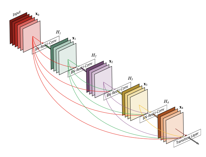
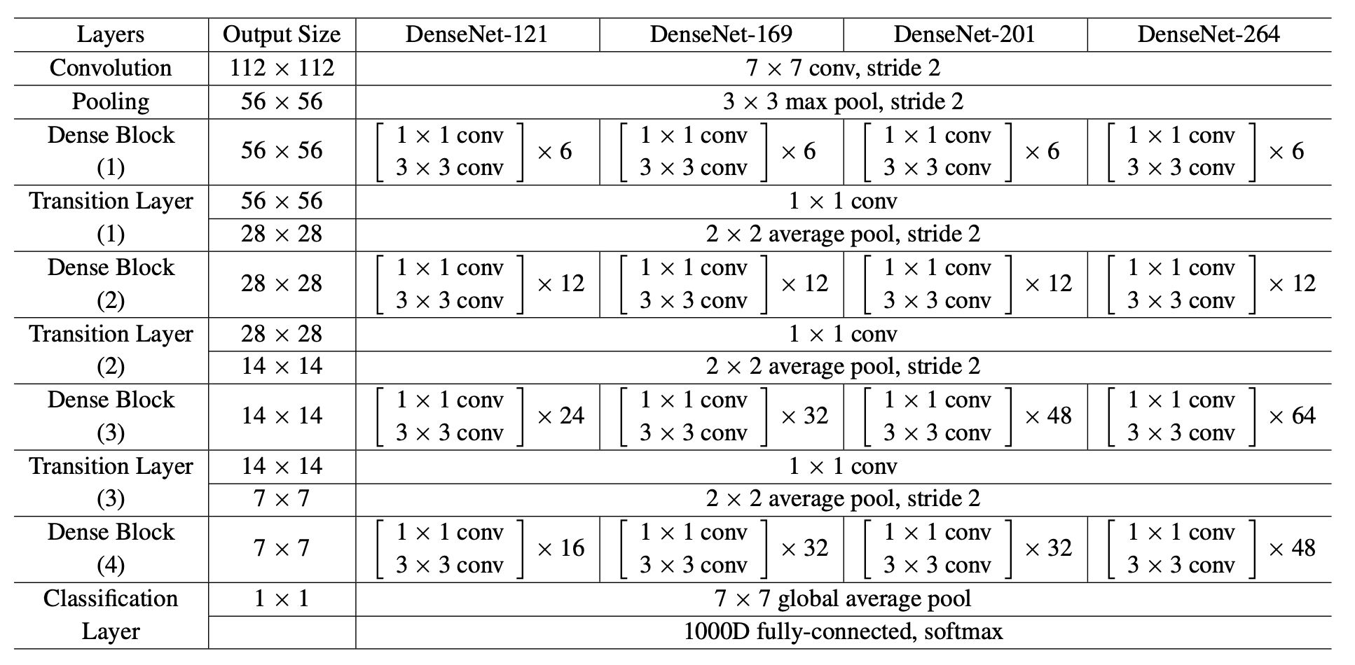
Dense Convolutional Network (DenseNet), connects each layer to every other layer in a feed-forward fashion. Whereas traditional convolutional networks with L layers have L connections - one between each layer and its subsequent layer - our network has L(L+1)/2 direct connections. For each layer, the feature-maps of all preceding layers are used as inputs, and its own feature-maps are used as inputs into all subsequent layers. DenseNets have several compelling advantages: they alleviate the vanishing-gradient problem, strengthen feature propagation, encourage feature reuse, and substantially reduce the number of parameters.
The 1-crop error rates on the imagenet dataset with the pretrained model are listed below.
| Model structure | Top-1 error | Top-5 error |
|---|---|---|
| densenet121 | 25.35 | 7.83 |
| densenet169 | 24.00 | 7.00 |
| densenet201 | 22.80 | 6.43 |
| densenet161 | 22.35 | 6.20 |


